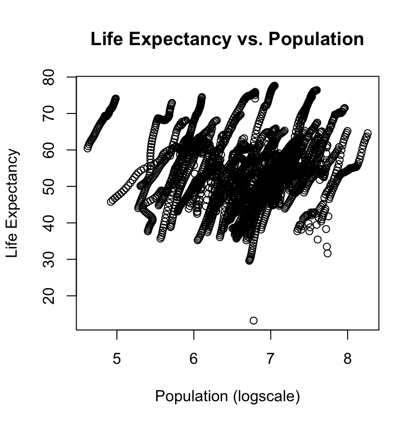
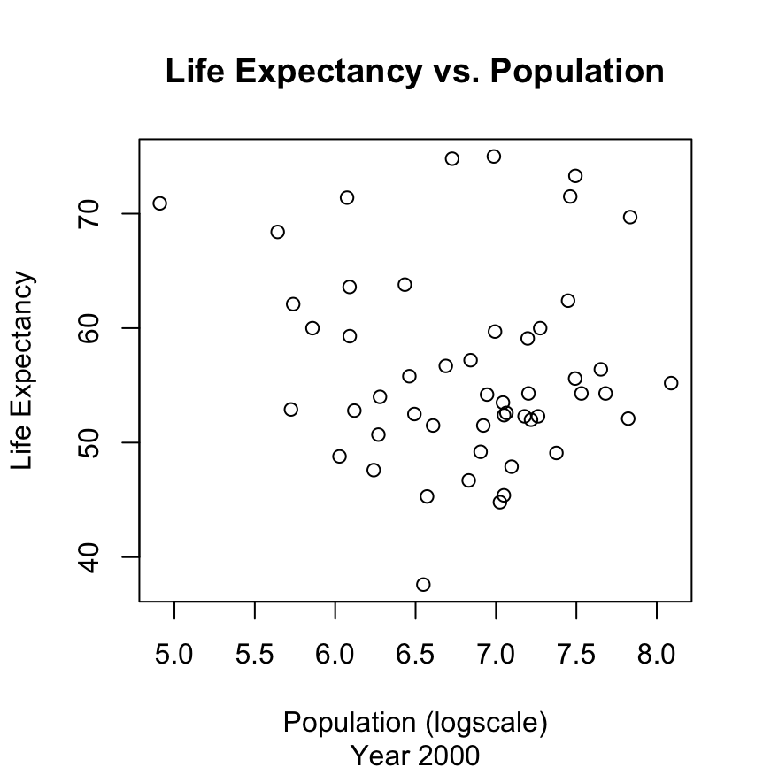
plot(log10(population_lifeexpec2000Spopulation), infmortality_lifeexpec2000$life_expectancy,
  main = "Life Expectancy vs. Population",
  xlab = "Population (logscale)",
  ylab = "Life Expectancy",
  sub = "Year 2000")
simple model fits
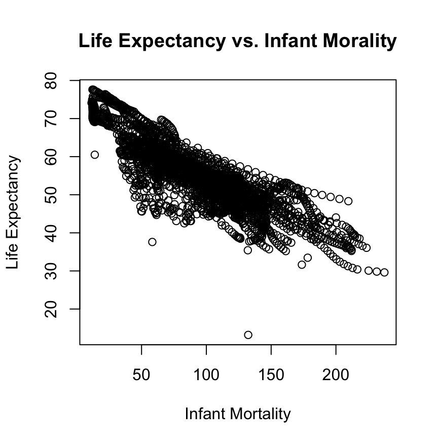
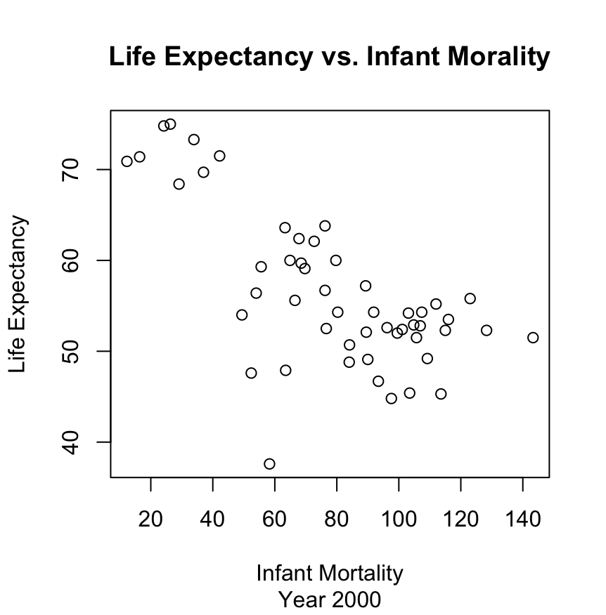
fits model with infant mortality as predictor pulling data from africadata_y2000
fit1 <- lm(life_expectancy ~ infant_mortality, data = africadata_y2000)
fits model with population size as predictor pulling data from africadata_y2000
fit2 <- lm(life_expectancy ~ population, data = africadata_y2000)
summary(fit1) - outputs stats summary for fit 1
summary(fit2) - outputs stats summary for fit 2
summary(fit1)
summary(fit2)
based on the p-values for each fit, fit 1 is a better model for the data.
This section is contributed by Ranni Tewfik.
This exercise uses the “us_contagious_diseases” dataset from the “dslabs” package. The dataset provides information on contagious diseases in the U.S. by state, year, and disease. There are six variables in the dataset: disease, state, year, weeks reporting, count, and population.
Part 1 - Loading and Checking Data
#Load the required packageslibrary(dslabs)library(dplyr)
Attaching package: 'dplyr'
The following objects are masked from 'package:stats':

    filter, lag
The following objects are masked from 'package:base':

    intersect, setdiff, setequal, union
library(ggplot2)#Look at help file for "us_contagious_diseases"help(us_contagious_diseases)#Get an overview of data structurestr(us_contagious_diseases)
#Get a summary of datasummary(us_contagious_diseases)
        disease            state            year      weeks_reporting
 Hepatitis A:2346   Alabama   :  315   Min.   :1928   Min.   : 0.00
 Measles    :3825   Alaska    :  315   1st Qu.:1950   1st Qu.:31.00
 Mumps      :1785   Arizona   :  315   Median :1975   Median :46.00
 Pertussis  :2856   Arkansas  :  315   Mean   :1971   Mean   :37.38
 Polio      :2091   California:  315   3rd Qu.:1990   3rd Qu.:50.00
 Rubella    :1887   Colorado  :  315   Max.   :2011   Max.   :52.00
 Smallpox   :1275   (Other)   :14175
     count          population
 Min.   :     0   Min.   :   86853
 1st Qu.:     7   1st Qu.: 1018755
 Median :    69   Median : 2749249
 Mean   :  1492   Mean   : 4107584
 3rd Qu.:   525   3rd Qu.: 4996229
 Max.   :132342   Max.   :37607525
                  NA's   :214
#Determine the type of object "us_contagious_diseases" isclass(us_contagious_diseases)
[1] "data.frame"
Part 2 - Processing Data
#Assign only Pertussis and Georgia in "us_contagious_diseases" to a new objectgeorgia <-subset(us_contagious_diseases, disease =="Pertussis"& state =="Georgia")#Get an overview of data structure and data summary for "georgia"str(georgia)
        disease          state         year      weeks_reporting
 Hepatitis A: 0   Georgia   :56   Min.   :1938   Min.   : 2.00
 Measles    : 0   Alabama   : 0   1st Qu.:1952   1st Qu.:39.00
 Mumps      : 0   Alaska    : 0   Median :1984   Median :46.50
 Pertussis  :56   Arizona   : 0   Mean   :1978   Mean   :41.75
 Polio      : 0   Arkansas  : 0   3rd Qu.:1997   3rd Qu.:49.25
 Rubella    : 0   California: 0   Max.   :2011   Max.   :52.00
 Smallpox   : 0   (Other)   : 0
     count          population
 Min.   :   2.0   Min.   :3066678
 1st Qu.:  27.0   1st Qu.:3518196
 Median :  58.0   Median :5776280
 Mean   : 346.0   Mean   :5898795
 3rd Qu.: 571.5   3rd Qu.:7688876
 Max.   :1922.0   Max.   :9830160
#Create a new object that only contains year and countgeorgia1 <- georgia %>%select("year", "count")#Create a new object that only contains population and countgeorgia2 <- georgia %>%select("population", "count")#Get an overview of data structure and data summary for "georgia1" and "georgia2"str(georgia1)
'data.frame':   56 obs. of  2 variables:
 $ year : num  1938 1939 1940 1941 1942 ...
 $ count: num  1922 1573 1114 1265 1288 ...
summary(georgia1)
      year          count
 Min.   :1938   Min.   :   2.0
 1st Qu.:1952   1st Qu.:  27.0
 Median :1984   Median :  58.0
 Mean   :1978   Mean   : 346.0
 3rd Qu.:1997   3rd Qu.: 571.5
 Max.   :2011   Max.   :1922.0
str(georgia2)
'data.frame':   56 obs. of  2 variables:
 $ population: num  3066678 3095013 3123723 3152430 3181234 ...
 $ count     : num  1922 1573 1114 1265 1288 ...
summary(georgia2)
   population          count
 Min.   :3066678   Min.   :   2.0
 1st Qu.:3518196   1st Qu.:  27.0
 Median :5776280   Median :  58.0
 Mean   :5898795   Mean   : 346.0
 3rd Qu.:7688876   3rd Qu.: 571.5
 Max.   :9830160   Max.   :1922.0
Part 3 - Plotting
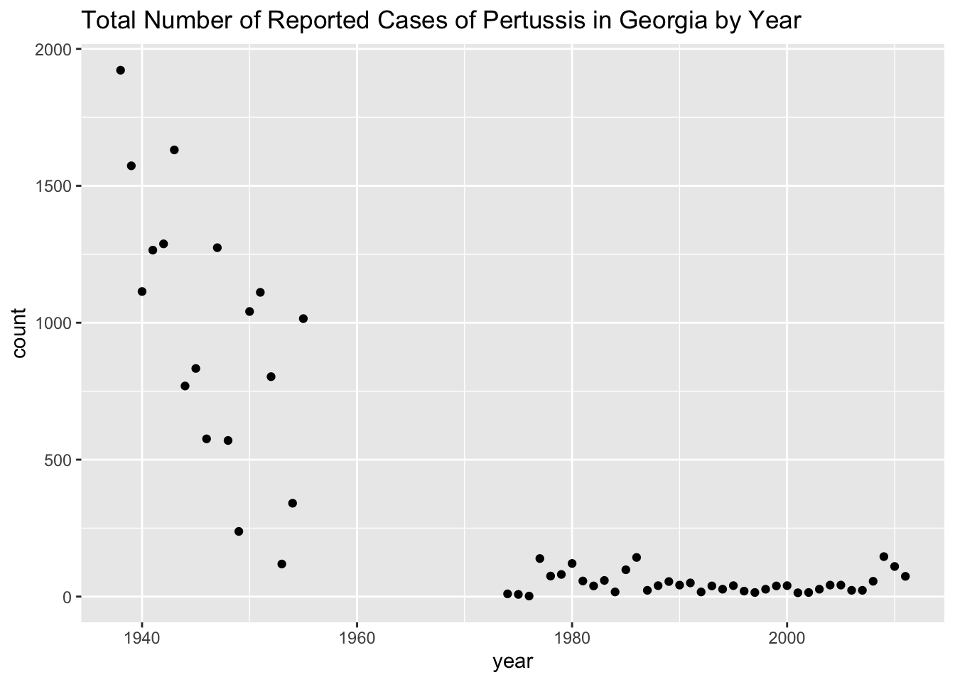
#Plot count as a function of yearggplot(georgia1, aes(x = year, y = count)) +geom_point() +ggtitle("Total Number of Reported Cases of Pertussis in Georgia by Year")
There is a negative correlation between year and count to a certain point in the plot, and then there is a break in the data (no available data for 1956-1973). After that point, there seems to be no correlation between year and count.
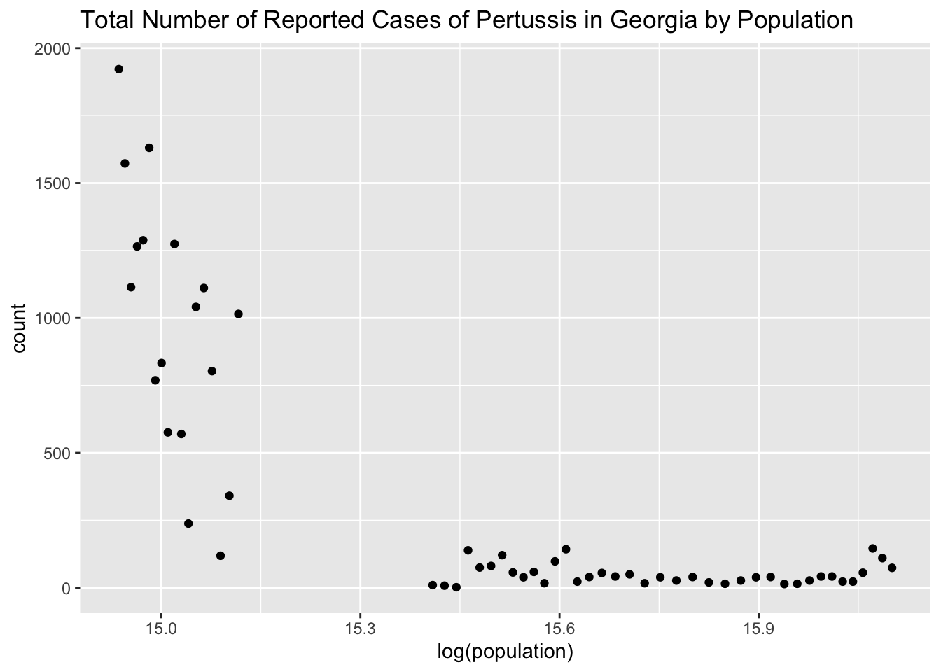
#Plot count as a function of populationggplot(georgia2, aes(x =log(population), y = count)) +geom_point() +ggtitle("Total Number of Reported Cases of Pertussis in Georgia by Population")
Similar to the previous plot, there is a negative correlation between population and count to a certain point. However, there is a noticeable break in the data, and there seems to be no correlation between population and count after that point. This is because no data is available for the years 1956-1973.
Part 4 - More Data Processing
#Create a new object by extracting only the data for the years after 1973 from "georgia"georgia3 <- georgia[(georgia$year >=1974),]#Get an overview of data structure and data summary for "africadata3"str(georgia3)
        disease          state         year      weeks_reporting
 Hepatitis A: 0   Georgia   :38   Min.   :1974   Min.   : 2.00
 Measles    : 0   Alabama   : 0   1st Qu.:1983   1st Qu.:34.75
 Mumps      : 0   Alaska    : 0   Median :1992   Median :42.50
 Pertussis  :38   Arizona   : 0   Mean   :1992   Mean   :38.45
 Polio      : 0   Arkansas  : 0   3rd Qu.:2002   3rd Qu.:47.75
 Rubella    : 0   California: 0   Max.   :2011   Max.   :51.00
 Smallpox   : 0   (Other)   : 0
     count          population
 Min.   :  2.00   Min.   :4920562
 1st Qu.: 23.00   1st Qu.:5753480
 Median : 40.00   Median :6852235
 Mean   : 49.87   Mean   :7111873
 3rd Qu.: 58.50   3rd Qu.:8480435
 Max.   :146.00   Max.   :9830160
Part 5 - More Plotting
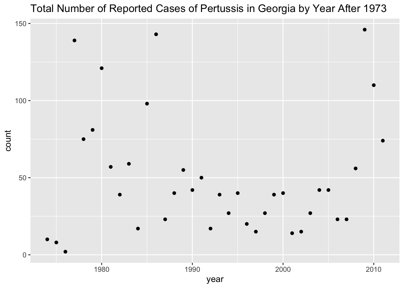
#Plot count as a function of year for the years after 1973ggplot(georgia3, aes(x = year, y = count)) +geom_point() +ggtitle("Total Number of Reported Cases of Pertussis in Georgia by Year After 1973")
There is no noticeable correlation between year and count after 1973.
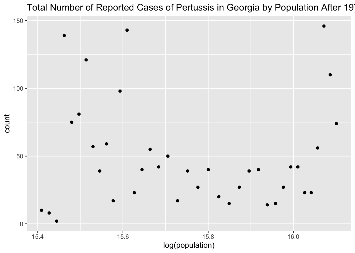
#Plot count as a function of population for the years after 1973ggplot(georgia3, aes(x =log(population), y = count)) +geom_point() +ggtitle("Total Number of Reported Cases of Pertussis in Georgia by Population After 1973")
There is no noticeable correlation between population and count after 1973.
Part 6 - Simple Model Fits
#Fit count as the outcome and year as the predictorfit1 <-glm(count ~ year, data = georgia3, family =poisson(link ="log"))summary(fit1)
Call:
glm(formula = count ~ year, family = poisson(link = "log"), data = georgia3)

Coefficients:
             Estimate Std. Error z value Pr(>|z|)
(Intercept)  8.810681   4.174343   2.111   0.0348 *
year        -0.002460   0.002095  -1.174   0.2404
---
Signif. codes:  0 '***' 0.001 '**' 0.01 '*' 0.05 '.' 0.1 ' ' 1

(Dispersion parameter for poisson family taken to be 1)

    Null deviance: 1026.6  on 37  degrees of freedom
Residual deviance: 1025.3  on 36  degrees of freedom
AIC: 1235.8

Number of Fisher Scoring iterations: 5
After 1973, count is not significantly associated with year (p-value = 0.24).
#Fit count as the outcome and population as the predictorfit2 <-glm(count ~ population, data = georgia3, family =poisson(link ="log"))summary(fit2)
Call:
glm(formula = count ~ population, family = poisson(link = "log"),
    data = georgia3)

Coefficients:
              Estimate Std. Error z value Pr(>|z|)
(Intercept)  4.007e+00  1.089e-01  36.801   <2e-16 ***
population  -1.370e-08  1.503e-08  -0.912    0.362
---
Signif. codes:  0 '***' 0.001 '**' 0.01 '*' 0.05 '.' 0.1 ' ' 1

(Dispersion parameter for poisson family taken to be 1)

    Null deviance: 1026.6  on 37  degrees of freedom
Residual deviance: 1025.8  on 36  degrees of freedom
AIC: 1236.3

Number of Fisher Scoring iterations: 5
After 1973, count is not significantly associated with population (p-value = 0.36).