PATRICK KAGGWA contributed to this exercise.
Summary/Abstract
The Data Analysis exercise for Module 2 was completed in 3 parts.
Part 1 - adding two additional variables and their values to provided data sheet
Part 2 - cleaning and processing of data (performed by Patrick Kaggwa)
Part 3 - data analysis using provided linear analysis models
Introduction
General Background Information
This exercise was done as part of an assignment and is educational in nature. The premise of the assignment was the cleaning, processing, and analysis of a provided “unclean” data set via manipulation with R and RStudio. The exercise was also meant to encourage collaboration between classmates, in preparation for future collaboration involving scientific data.
Description of data and data source
Data included variables of ‘height’, ‘weight’, ‘gender’, ‘age’ and ‘hair color’. Each variable had 14 associated values which were either numeric or categorical.
The data was provided via Andreas Handel and Liza Hall.
Methods
Data acquisition
Data for ‘Height’, ‘Weight’, and ‘Gender’ were provided by Andreas Handel.
Data for ‘Age’ and ‘Hair Color’ were provided by Liza Hall, and were chosen using random generators available online (age generator).
Data import and cleaning
This part of the exercise was done by Patrick Kaggwa. All files can be found on Github in the ‘starter-analysis-exercise’ folder.
Data was imported, processed, and cleaned in RStudio using the following script:
---
title: "An example cleaning script"
author: "Patrick Kaggwa"
date: "2023-01-03"
output: html_document
---
# Processing script
This Quarto file contains a mix of code and explanatory text to illustrate a simple data processing/cleaning setup.
# Setup
Load needed packages. make sure they are installed.
::: {.cell}
```{.r .cell-code}
library(readxl) #for loading Excel files
library(dplyr) #for data processing/cleaning
```
::: {.cell-output .cell-output-stderr}
```
Attaching package: 'dplyr'
```
:::
::: {.cell-output .cell-output-stderr}
```
The following objects are masked from 'package:stats':
filter, lag
```
:::
::: {.cell-output .cell-output-stderr}
```
The following objects are masked from 'package:base':
intersect, setdiff, setequal, union
```
:::
```{.r .cell-code}
library(tidyr) #for data processing/cleaning
library(skimr) #for nice visualization of data
library(here) #to set paths
```
:::
# Data loading
Note that for functions that come from specific packages (instead of base R), I often specify both package and function like so:
package::function() that's not required one could just call the function specifying the package makes it clearer where the function "lives",
but it adds typing. You can do it either way.
::: {.cell}
```{.r .cell-code}
# path to data
# note the use of the here() package and not absolute paths
data_location <- here::here("starter-analysis-exercise","data","raw-data","exampledata2.xlsx")
rawdata <- readxl::read_excel(data_location)
```
:::
# Check data
First we can look at the codebook
::: {.cell}
```{.r .cell-code}
codebook <- readxl::read_excel(data_location, sheet ="Codebook")
print(codebook)
```
::: {.cell-output .cell-output-stdout}
```
# A tibble: 5 × 3
`Variable Name` `Variable Definition` `Allowed Values`
<chr> <chr> <chr>
1 Height height in centimeters numeric value >…
2 Weight weight in kilograms numeric value >…
3 Gender identified gender (male/female/other) M/F/O/NA
4 Age age in years numeric value >0
5 Hair Color hair color (black, brown, blonde, red, other) Blk, Bro, Bln, …
```
:::
:::
Several ways of looking at the data
::: {.cell}
```{.r .cell-code}
dplyr::glimpse(rawdata)
```
::: {.cell-output .cell-output-stdout}
```
Rows: 14
Columns: 5
$ Height <chr> "180", "175", "sixty", "178", "192", "6", "156", "166", "…
$ Weight <dbl> 80, 70, 60, 76, 90, 55, 90, 110, 54, 7000, NA, 45, 55, 50
$ Gender <chr> "M", "O", "F", "F", "NA", "F", "O", "M", "N", "M", "F", "…
$ Age <dbl> 26, 41, 58, 18, 58, 59, 24, 30, 20, 57, 40, 41, 57, 43
$ `Hair Color` <chr> "Bro", "Bro", "Bro", "Oth", "Bro", "Bln", "Blk", "Bro", "…
```
:::
```{.r .cell-code}
summary(rawdata)
```
::: {.cell-output .cell-output-stdout}
```
Height Weight Gender Age
Length:14 Min. : 45.0 Length:14 Min. :18.00
Class :character 1st Qu.: 55.0 Class :character 1st Qu.:27.00
Mode :character Median : 70.0 Mode :character Median :41.00
Mean : 602.7 Mean :40.86
3rd Qu.: 90.0 3rd Qu.:57.00
Max. :7000.0 Max. :59.00
NA's :1
Hair Color
Length:14
Class :character
Mode :character
```
:::
```{.r .cell-code}
head(rawdata)
```
::: {.cell-output .cell-output-stdout}
```
# A tibble: 6 × 5
Height Weight Gender Age `Hair Color`
<chr> <dbl> <chr> <dbl> <chr>
1 180 80 M 26 Bro
2 175 70 O 41 Bro
3 sixty 60 F 58 Bro
4 178 76 F 18 Oth
5 192 90 NA 58 Bro
6 6 55 F 59 Bln
```
:::
```{.r .cell-code}
skimr::skim(rawdata)
```
::: {.cell-output-display}
Table: Data summary
| | |
|:------------------------|:-------|
|Name |rawdata |
|Number of rows |14 |
|Number of columns |5 |
|_______________________ | |
|Column type frequency: | |
|character |3 |
|numeric |2 |
|________________________ | |
|Group variables |None |
**Variable type: character**
|skim_variable | n_missing| complete_rate| min| max| empty| n_unique| whitespace|
|:-------------|---------:|-------------:|---:|---:|-----:|--------:|----------:|
|Height | 0| 1| 1| 5| 0| 13| 0|
|Gender | 0| 1| 1| 2| 0| 5| 0|
|Hair Color | 0| 1| 3| 3| 0| 5| 0|
**Variable type: numeric**
|skim_variable | n_missing| complete_rate| mean| sd| p0| p25| p50| p75| p100|hist |
|:-------------|---------:|-------------:|------:|-------:|--:|---:|---:|---:|----:|:-----|
|Weight | 1| 0.93| 602.69| 1922.25| 45| 55| 70| 90| 7000|▇▁▁▁▁ |
|Age | 0| 1.00| 40.86| 15.25| 18| 27| 41| 57| 59|▆▂▅▂▇ |
:::
:::
# Cleaning
By inspecting the data as done above, we find some problems that need addressing:
First, there is an entry for height which says "sixty" instead of a number.
Does that mean it should be a numeric 60? It somehow doesn't make sense since the weight is 60kg, which can't happen for a 60cm person (a baby).
Since we don't know how to fix this, we might decide to remove the person. This "sixty" entry also turned all Height entries into characters instead of numeric. That conversion to character also means that our summary function isn't very meaningful. So let's fix that first.
::: {.cell}
```{.r .cell-code}
d1 <- rawdata %>% dplyr::filter( Height != "sixty" ) %>%
dplyr::mutate(Height = as.numeric(Height))
skimr::skim(d1)
```
::: {.cell-output-display}
Table: Data summary
| | |
|:------------------------|:----|
|Name |d1 |
|Number of rows |13 |
|Number of columns |5 |
|_______________________ | |
|Column type frequency: | |
|character |2 |
|numeric |3 |
|________________________ | |
|Group variables |None |
**Variable type: character**
|skim_variable | n_missing| complete_rate| min| max| empty| n_unique| whitespace|
|:-------------|---------:|-------------:|---:|---:|-----:|--------:|----------:|
|Gender | 0| 1| 1| 2| 0| 5| 0|
|Hair Color | 0| 1| 3| 3| 0| 5| 0|
**Variable type: numeric**
|skim_variable | n_missing| complete_rate| mean| sd| p0| p25| p50| p75| p100|hist |
|:-------------|---------:|-------------:|------:|-------:|--:|------:|---:|---:|----:|:-----|
|Height | 0| 1.00| 151.62| 46.46| 6| 154.00| 165| 175| 192|▁▁▁▂▇ |
|Weight | 1| 0.92| 647.92| 2000.48| 45| 54.75| 73| 90| 7000|▇▁▁▁▁ |
|Age | 0| 1.00| 39.54| 15.02| 18| 26.00| 41| 57| 59|▇▂▆▂▇ |
:::
```{.r .cell-code}
hist(d1$Height)
```
::: {.cell-output-display}
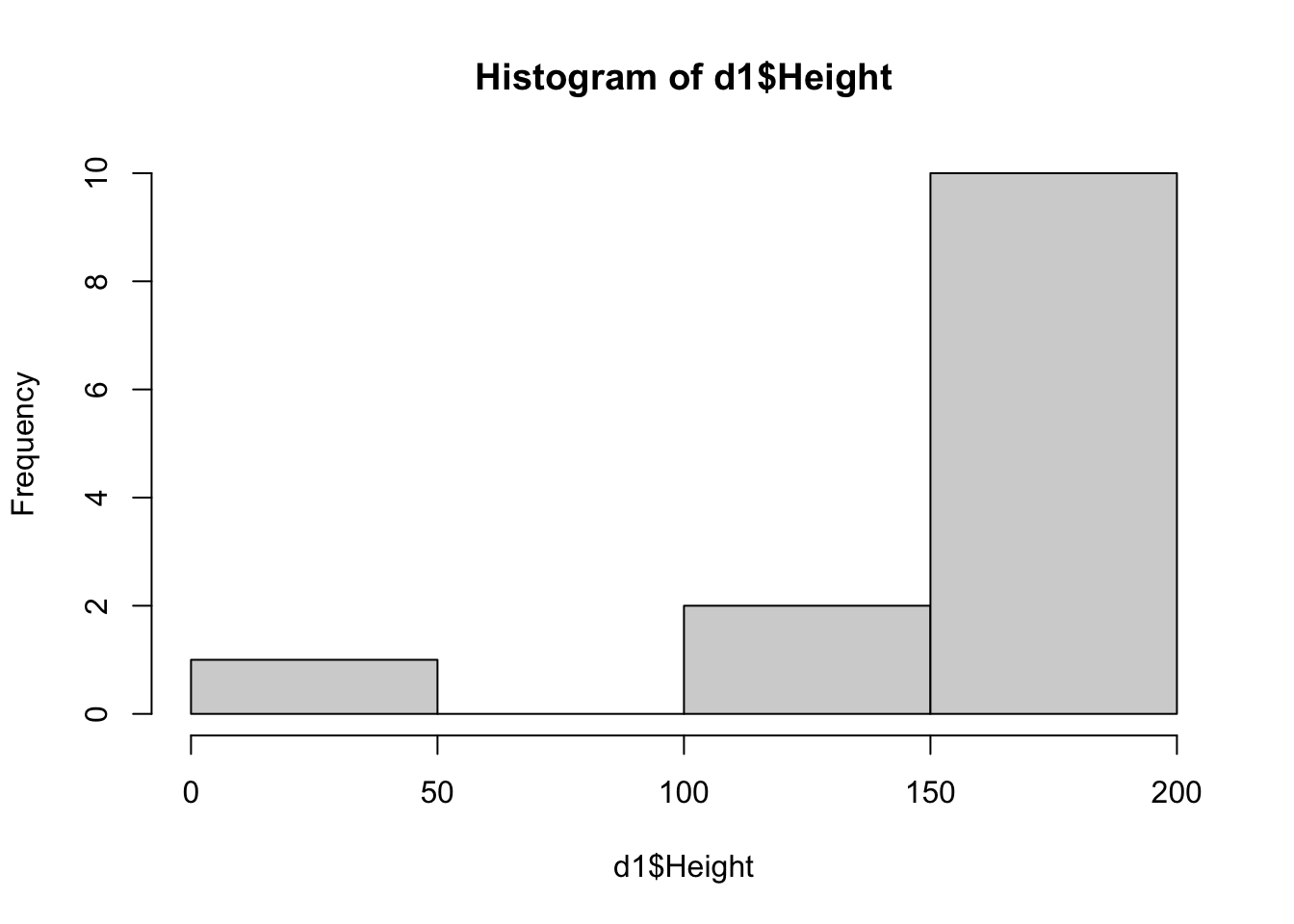{width=672}
:::
:::
Now we see that there is one person with a height of 6. That could be a typo, or someone mistakenly entered their height in feet. Since we unfortunately don't know, we might need to remove this person, which we'll do here.
::: {.cell}
```{.r .cell-code}
d2 <- d1 %>% dplyr::mutate( Height = replace(Height, Height=="6",round(6*30.48,0)) )
skimr::skim(d2)
```
::: {.cell-output-display}
Table: Data summary
| | |
|:------------------------|:----|
|Name |d2 |
|Number of rows |13 |
|Number of columns |5 |
|_______________________ | |
|Column type frequency: | |
|character |2 |
|numeric |3 |
|________________________ | |
|Group variables |None |
**Variable type: character**
|skim_variable | n_missing| complete_rate| min| max| empty| n_unique| whitespace|
|:-------------|---------:|-------------:|---:|---:|-----:|--------:|----------:|
|Gender | 0| 1| 1| 2| 0| 5| 0|
|Hair Color | 0| 1| 3| 3| 0| 5| 0|
**Variable type: numeric**
|skim_variable | n_missing| complete_rate| mean| sd| p0| p25| p50| p75| p100|hist |
|:-------------|---------:|-------------:|------:|-------:|---:|------:|---:|---:|----:|:-----|
|Height | 0| 1.00| 165.23| 16.52| 133| 155.00| 166| 178| 192|▂▇▆▆▃ |
|Weight | 1| 0.92| 647.92| 2000.48| 45| 54.75| 73| 90| 7000|▇▁▁▁▁ |
|Age | 0| 1.00| 39.54| 15.02| 18| 26.00| 41| 57| 59|▇▂▆▂▇ |
:::
:::
Height values seem ok now.
Now let's look at the `Weight` variable. There is a person with weight of 7000, which is impossible, and one person with missing weight.
To be able to analyze the data, we'll remove those individuals as well.
::: {.cell}
```{.r .cell-code}
d3 <- d2 %>% dplyr::filter(Weight != 7000) %>% tidyr::drop_na()
skimr::skim(d3)
```
::: {.cell-output-display}
Table: Data summary
| | |
|:------------------------|:----|
|Name |d3 |
|Number of rows |11 |
|Number of columns |5 |
|_______________________ | |
|Column type frequency: | |
|character |2 |
|numeric |3 |
|________________________ | |
|Group variables |None |
**Variable type: character**
|skim_variable | n_missing| complete_rate| min| max| empty| n_unique| whitespace|
|:-------------|---------:|-------------:|---:|---:|-----:|--------:|----------:|
|Gender | 0| 1| 1| 2| 0| 5| 0|
|Hair Color | 0| 1| 3| 3| 0| 4| 0|
**Variable type: numeric**
|skim_variable | n_missing| complete_rate| mean| sd| p0| p25| p50| p75| p100|hist |
|:-------------|---------:|-------------:|------:|-----:|---:|-----:|---:|---:|----:|:-----|
|Height | 0| 1| 167.09| 16.81| 133| 155.5| 166| 179| 192|▂▇▅▇▅ |
|Weight | 0| 1| 70.45| 20.65| 45| 54.5| 70| 85| 110|▇▂▃▃▂ |
|Age | 0| 1| 37.91| 15.40| 18| 25.0| 41| 50| 59|▇▂▃▂▆ |
:::
:::
Now checking the `Gender` variable. Gender should be a categorical/factor variable but is loaded as character. We can fix that with simple base R code to mix things up.
::: {.cell}
```{.r .cell-code}
d3$Gender <- as.factor(d3$Gender)
skimr::skim(d3)
```
::: {.cell-output-display}
Table: Data summary
| | |
|:------------------------|:----|
|Name |d3 |
|Number of rows |11 |
|Number of columns |5 |
|_______________________ | |
|Column type frequency: | |
|character |1 |
|factor |1 |
|numeric |3 |
|________________________ | |
|Group variables |None |
**Variable type: character**
|skim_variable | n_missing| complete_rate| min| max| empty| n_unique| whitespace|
|:-------------|---------:|-------------:|---:|---:|-----:|--------:|----------:|
|Hair Color | 0| 1| 3| 3| 0| 4| 0|
**Variable type: factor**
|skim_variable | n_missing| complete_rate|ordered | n_unique|top_counts |
|:-------------|---------:|-------------:|:-------|--------:|:----------------------|
|Gender | 0| 1|FALSE | 5|M: 4, F: 3, O: 2, N: 1 |
**Variable type: numeric**
|skim_variable | n_missing| complete_rate| mean| sd| p0| p25| p50| p75| p100|hist |
|:-------------|---------:|-------------:|------:|-----:|---:|-----:|---:|---:|----:|:-----|
|Height | 0| 1| 167.09| 16.81| 133| 155.5| 166| 179| 192|▂▇▅▇▅ |
|Weight | 0| 1| 70.45| 20.65| 45| 54.5| 70| 85| 110|▇▂▃▃▂ |
|Age | 0| 1| 37.91| 15.40| 18| 25.0| 41| 50| 59|▇▂▃▂▆ |
:::
:::
Now we see that there is another NA, but it's not `NA` from R, instead it was loaded as character and is now considered as a category.
Well proceed here by removing that individual with that NA entry. Since this keeps an empty category for Gender, I'm also using droplevels() to get rid of it.
::: {.cell}
```{.r .cell-code}
d4 <- d3 %>% dplyr::filter( !(Gender %in% c("NA","N")) ) %>% droplevels()
skimr::skim(d4)
```
::: {.cell-output-display}
Table: Data summary
| | |
|:------------------------|:----|
|Name |d4 |
|Number of rows |9 |
|Number of columns |5 |
|_______________________ | |
|Column type frequency: | |
|character |1 |
|factor |1 |
|numeric |3 |
|________________________ | |
|Group variables |None |
**Variable type: character**
|skim_variable | n_missing| complete_rate| min| max| empty| n_unique| whitespace|
|:-------------|---------:|-------------:|---:|---:|-----:|--------:|----------:|
|Hair Color | 0| 1| 3| 3| 0| 4| 0|
**Variable type: factor**
|skim_variable | n_missing| complete_rate|ordered | n_unique|top_counts |
|:-------------|---------:|-------------:|:-------|--------:|:----------------|
|Gender | 0| 1|FALSE | 3|M: 4, F: 3, O: 2 |
**Variable type: numeric**
|skim_variable | n_missing| complete_rate| mean| sd| p0| p25| p50| p75| p100|hist |
|:-------------|---------:|-------------:|------:|-----:|---:|---:|---:|---:|----:|:-----|
|Height | 0| 1| 165.67| 15.98| 133| 156| 166| 178| 183|▂▁▃▃▇ |
|Weight | 0| 1| 70.11| 21.25| 45| 55| 70| 80| 110|▇▂▃▂▂ |
|Age | 0| 1| 37.67| 14.35| 18| 26| 41| 43| 59|▇▂▅▂▅ |
:::
:::
All done, data is clean now.
Let's assign at the end to some final variable, this makes it easier to add further cleaning steps above.
::: {.cell}
```{.r .cell-code}
processeddata <- d4
```
:::
# Save data
Finally, we save the clean data as RDS file. I suggest you save your processed and cleaned data as RDS or RDA/Rdata files.
This preserves coding like factors, characters, numeric, etc. If you save as CSV, that information would get lost.
However, CSV is better for sharing with others since it's plain text. If you do CSV, you might want to write down somewhere what each variable is.
See here for some suggestions on how to store your processed data:
http://www.sthda.com/english/wiki/saving-data-into-r-data-format-rds-and-rdata
::: {.cell}
```{.r .cell-code}
save_data_location <- here::here("starter-analysis-exercise","data","processed-data","processeddata.rds")
saveRDS(processeddata, file = save_data_location)
```
:::
Note the use of the `here` package and `here` command to specify a path relative to the main project directory, that is the folder that contains the `.Rproj` file. Always use this approach instead of hard-coding file paths that only exist on your computer.
# Notes
Removing anyone observation with "faulty" or missing data is one approach. It's often not the best. based on your question and your analysis approach, you might want to do cleaning differently (e.g. keep observations with some missing information).Statistical analysis
Statistical analysis for Table 1 was done using the following code.
############################
#### Third model fit
# fit linear model using height as outcome, hair color and age as predictors

lmfit3 <- lm(Height ~ `Hair Color` + `Age`, mydata)

# place results from fit into a data frame with the tidy function
lmtable3 <- broom::tidy(lmfit3)

#look at fit results
print(lmtable3)

# save fit results table
table_file3 = here("starter-analysis-exercise","results", "tables-files", "resulttable3.rds")
saveRDS(lmtable3, file = table_file3)
Results
Figures and Tables
Figures were generated by Patrick Kaggwa, tables were produced by Liza Hall.
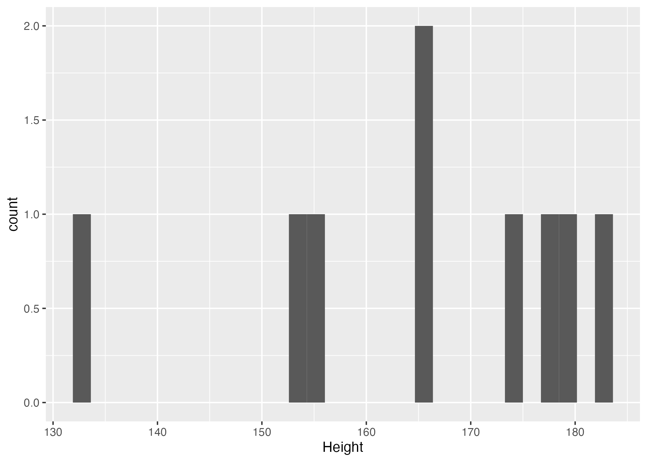
Figure 1. Height distribution histogram
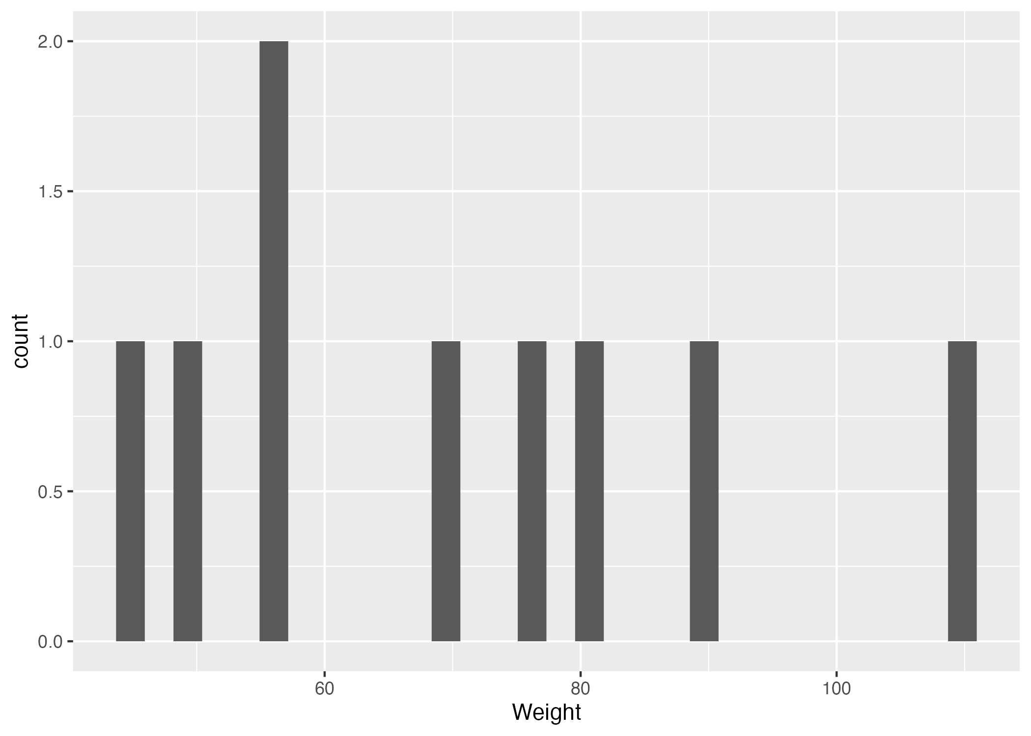
Figure 2. Weight distribution histogram
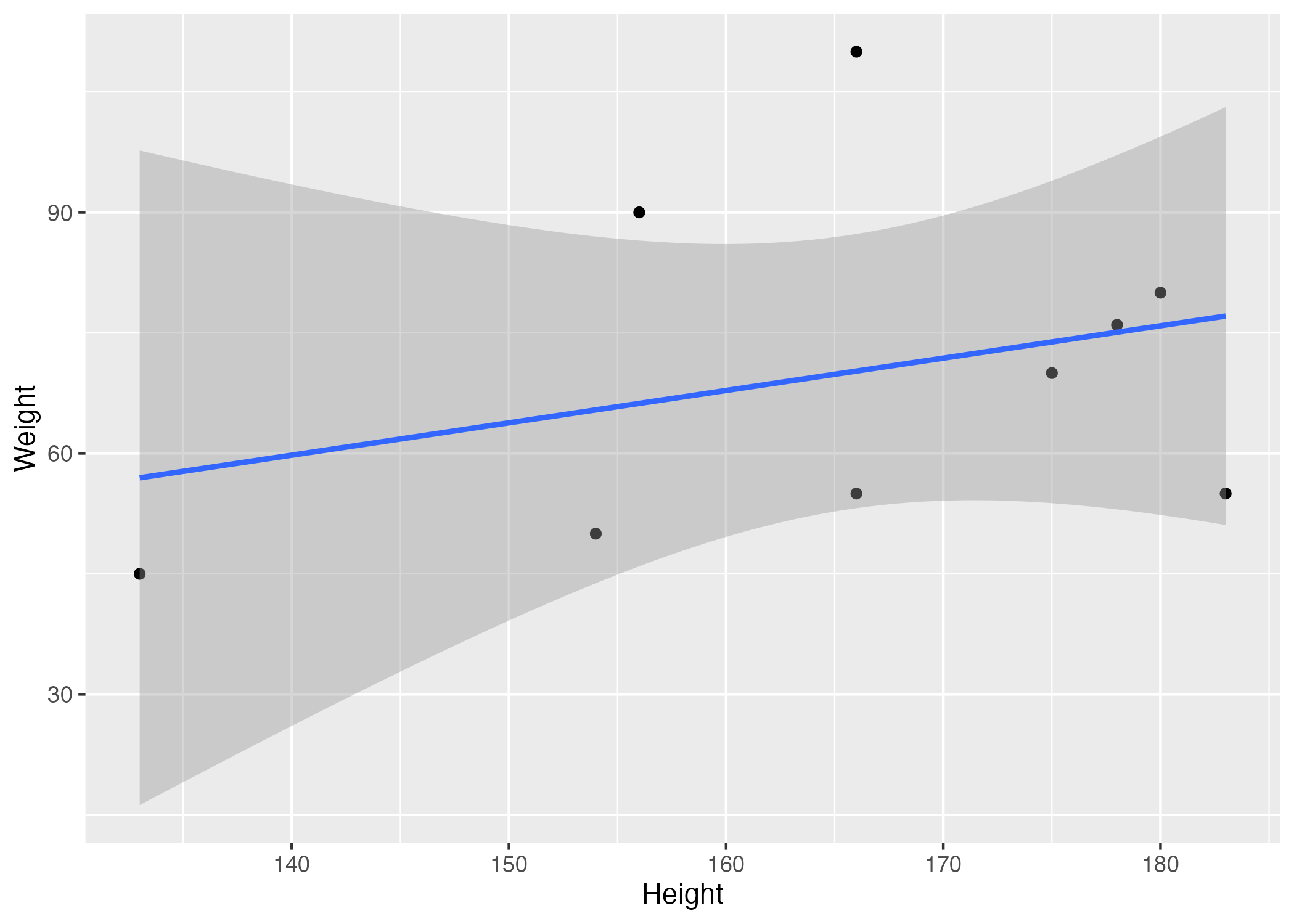
Figure 3. Scatter plot with linear regression fit depicting the relationship between height and weight
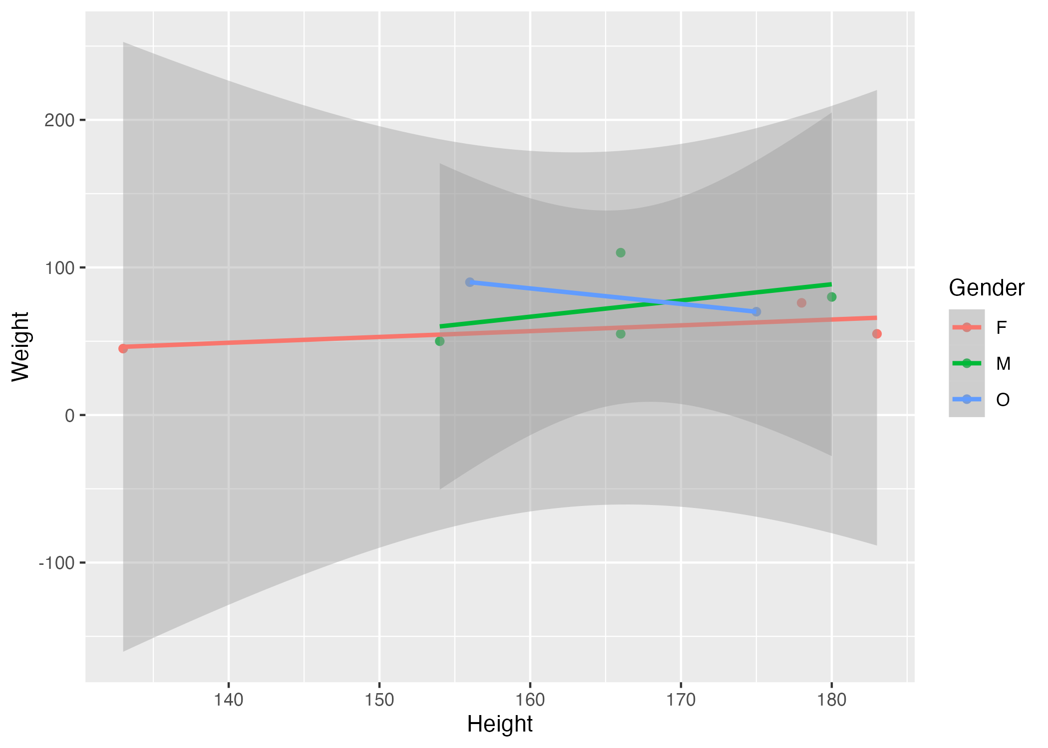
Figure 4. Scatter plot with gender-stratified linear regression fits illustrating the relationship between height and weight
A tibble 5x5
| term | estimate | std.error | statistic | p. value | |
| 1 | (Intercept) | 156. | 25.5 | 6.12 | 0.00367 |
| 2 | ‘Hair Color’ Bln | 2.06 | 30.0 | 0.0687 | 0.949 |
| 3 | ‘Hair Color’ Bro | 15.8 | 24.7 | 0.639 | 0.558 |
| 4 | ‘Hair Color’ Oth | 10.0 | 25.5 | 0.393 | 0.714 |
| 5 | Age | -0.00238 | 0.633 | -0.00376 | 0.997 |
Table 1. Table of outcomes from a fit linear model using height as outcome and hair color and age as predictors